surv <- standardize_data(dataType = 'Surveys', channel = dbutils::connect_to_database(server="NEFSC_pw_oraprod",uid="KGALLAGHER"))Building & Predicting Ensemble Species Distribution Models
Overview
The first step in the CVA2.0 workflow is to build the species distribution models. These will be the basis of the exposure, directionality, and possibly additional indicators from the CVA. These are what allow the calculations to be spatially explicit and account for species habitat use.
Within this workflow, there are three steps:
- Data preparation
- Building & Predicting Species Distribution Models
- Building & Predicting the Ensemble
The functions outlined below are designed to be run either sequentially or in parallel with the R parallelization method of your choice (doParallel and furrr are recommended) and can be run in loops across a list of species.
Data Preparation
Fisheries Data
The function standardize_data can be used to standardize provided csv files or pull NEFSC survey or observer data from NEFSC databases via ROracle. This can also be accomplished in R outside of the package, but standardize_data provides a single function to format data in a way that will be accepted by downstream functions. If you are pulling together data from a variety of sources, you will likely still need to manipulate data outside of this function to make sure that data are in a single csv file and that dates and times are in the correct format.
To pull NEFSC survey or observer data, a channel from the package dbutils must be provided:
To standardize CSV data, a file path to the csv file, as well as column names for station IDs; position (longitude/latitude); date; the column corresponding to the presence/absence, or count of the species; and species name.
neamap <- standardize_data(dataType = 'CSV', csv = "./Data/csvs/raw/NEAMAP_Tow_Catch_2025-08-14.csv", csvCols = c('station', 'lon', 'lat', 'date', 'present_absent', 'SCI_NAME'))This function results in a dataframe being transformed from this:
  X      ID TRIP_NUMBER.x HAUL_NUMBER.x AREA_FISHED SET_BEGIN_DATE SET_END_DATE
1 1 44473.1         44473             1        3674      4/11/2010    4/11/2010
2 2 44473.2         44473             2        3674      4/11/2010    4/11/2010
3 3 44473.3         44473             3        3674      4/11/2010    4/11/2010
4 4 44473.5         44473             5        3674      4/11/2010    4/11/2010
5 5 44473.5         44473             5        3674      4/11/2010    4/11/2010
6 6 44473.5         44473             5        3674      4/11/2010    4/11/2010
  HAUL_BEGIN_DATE HAUL_END_DATE SET_BEGIN_LAT_CONV SET_BEGIN_LONG_CONV
1       4/11/2010     4/11/2010             36.068             -74.921
2       4/11/2010     4/11/2010             36.050             -74.909
3       4/11/2010     4/11/2010             36.042             -74.942
4       4/11/2010     4/11/2010             36.002             -74.975
5       4/11/2010     4/11/2010             36.002             -74.975
6       4/11/2010     4/11/2010             36.002             -74.975
  HAUL_BEGIN_LAT_CONV HAUL_BEGIN_LONG_CONV HAUL_END_LAT_CONV HAUL_END_LONG_CONV
1              36.063               74.921            36.065             74.936
2              36.049               74.909            36.050             74.913
3              36.044               74.941            36.044             74.945
4              36.007               74.975            36.004             74.975
5              36.007               74.975            36.004             74.975
6              36.007               74.975            36.004             74.975
  SET_DURATION HAUL_DURATION_HOURS GEAR_SOAK_HOURS  startDate VESSEL_ID
1         0.07                0.90            3.08 2010-04-11    926397
2         0.07                0.32            0.80 2010-04-11    926397
3         0.03                0.18            0.48 2010-04-11    926397
4         0.05                0.27            0.50 2010-04-11    926397
5         0.05                0.27            0.50 2010-04-11    926397
6         0.05                0.27            0.50 2010-04-11    926397
  TRIP_NUMBER.y HAUL_NUMBER.y         SPECIES_NAME NUM_FISH SPECIES_ON_LIST
1         44473             1             BLUEFISH      363               1
2         44473             2             BLUEFISH       64               1
3         44473             3             BLUEFISH        7               1
4         44473             5             BLUEFISH       14               1
5         44473             5 SHARK DOGFISH SMOOTH        3               0
6         44473             5  SHARK DOGFISH SPINY        6               0
To this:
  X       time month year   towID     lon    lat       date count
1 1 2010-04-11     4 2010 44473.1 -74.921 36.068 2010-04-11   363
2 2 2010-04-11     4 2010 44473.2 -74.909 36.050 2010-04-11    64
3 3 2010-04-11     4 2010 44473.3 -74.942 36.042 2010-04-11     7
4 4 2010-04-11     4 2010 44473.5 -74.975 36.002 2010-04-11    14
5 5 2010-04-11     4 2010 44473.5 -74.975 36.002 2010-04-11     3
6 6 2010-04-11     4 2010 44473.5 -74.975 36.002 2010-04-11     6
                  name
1             BLUEFISH
2             BLUEFISH
3             BLUEFISH
4             BLUEFISH
5 SHARK DOGFISH SMOOTH
6  SHARK DOGFISH SPINY
To ensure that fisheries and environmental data are on the same scale, and to convert any abundance data to presence/absence, the fisheries csvs produced by standardize_data are then converted into rasters of effort/presence/absence with the function create_rast. While the source datasets are generated for the entire dataset, one rasterStack is produced for each target species and data source. create_rast produces rasters with the same resolution as the environmental data where values range from 0 to 2, where 0 means that no effort was present in the grid cell, 1 means that there was fishing effort but the target species was not caught, and 2 indicates that the target species was caught in that grid cell.
Users must provide the standardized csv files generated by standardize_data, a link to a netcdf file that the desired grid and timesteps can be extracted from, the start date of the timeseries, and a vector of alternate names for the target species to account for any differences in species names across data sources. The user must also indicate if the data come from fisheries independent (surveys) or dependent sources (observer or logbook programs). If data come from fisheries dependent sources, then a threshold is applied before the raster is created, following McHenry et al 2019; rasters are only created if the species is present at least 30 times throughout the dataset.
rast <- create_rast(data = csv, isObs = FALSE, grid = "http://psl.noaa.gov/thredds/dodsC/Projects/CEFI/regional_mom6/cefi_portal/northwest_atlantic/full_domain/hindcast/monthly/regrid/r20250715/tob.nwa.full.hcast.monthly.regrid.r20250715.199301-202312.nc", origin = '1993-01-01', targetVec = "Atlantic cod ,ATLANTIC COD ,Gadus morhua,Cod Atlantic,GADUS MORHUA") #example to make raster for Atlantic CodThe resulting rasterStack will have a range from 0-2 with a number of layers equal to the length of the timeseries. Below is an example layer from the produced rasterStack for Atlantic Cod from the NEFSC survey data. 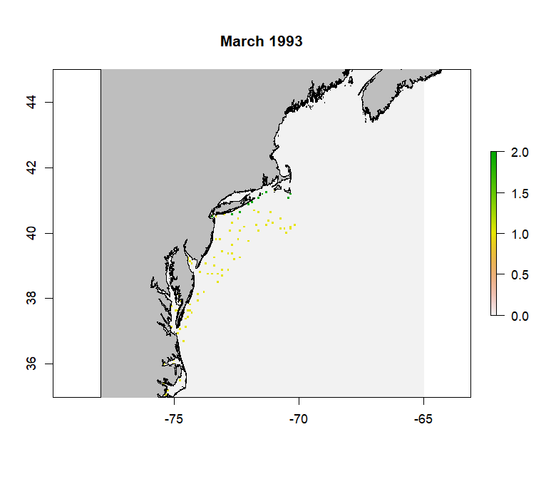
The wrapper function saveRast is provided for create_rast. This wrapper function provides logging functionality to keep track of progress, which is especially helpful if running the code in parallel, and also adds a skip functionality to skip making the raster if it already exists for that species and data source. It also saves the resulting rasterStack in the input_rasters directory within the species-specific folder in the working directory.
Here is an example of using saveRast in parallel using the package furrr with future_pmap:
plan(multisession, workers = 5)
future_pmap(list(..1 = argsList$csvName, ..2 = argsList$spp, ..3 = altNames, ..4 = argsList$skip, ..5 = argsList$isObs), ~ saveRast(csvName = ..1, spp = ..2, sppNames = ..3, skip = ..4, isObs = ..5, grid = "http://psl.noaa.gov/thredds/dodsC/Projects/CEFI/regional_mom6/cefi_portal/northwest_atlantic/full_domain/hindcast/monthly/regrid/r20230520/tob.nwa.full.hcast.monthly.regrid.r20230520.199301-201912.nc", origin = '1993-01-01'), .progress = T)
plan(sequential)
Where argsList is a dataframe with a row for each desired call of saveRast, and a column associated with most arguments for saveRast and create_rast. This is generated using tidyr::expand_grid to create a dataframe of every combination of target species and data sources.
create_rast creates a seperate rasterStack for each species, which is saved to the species-specific input_rasters folder bv the saveRast wrapper function. This allows the user to examine the raster for each data source independently to ensure that it meets expectations. Before these can be matched with the environmental data, the rasters must be combined into a single rasterStack, while maintaining the 0-2 range to document presences, absences, and lack of effort. This is done with the merge_rasts and associated combineSave wrapper function. The combineSave wrapper function, in addition to providing logging and skip functionality, also automatically creates a list of raster objects in the input_rasters folder for the merge_rasts function.
combinedRasts <- merge_rasts(rasts)
#where rasts is a list of rasterStacks to combine
The wrapper function combineSave is similar to saveRast where is provides logging and skip functionality. This function also handles creating the list of rasterStacks necessary to provide to create_rast. It is also written to be run in parallel:
options(future.globals.maxSize = Inf)
plan(multisession, workers = 5)
combs <- future_pmap(list(..1 = args$name, ..2 = args$skip), ~ combineSave(name = ..1, skip = ..2), .progress = T)
plan(sequential)
The resulting combined rasterStack will retain the range from 0-2 with a number of layers equal to the length of the timeseries. It works by retaining the maximum value in a grid cell across a given layer (which represent different timestamps) of the provided rasterStacks. Below is an example layer from the merged rasterStack for Atlantic Cod from the NEFSC survey data. 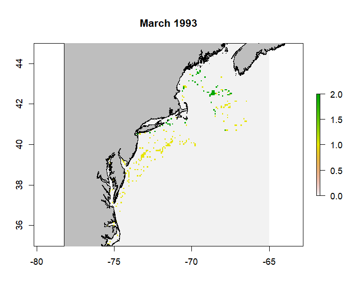
Environmental Data
The example below illustrates how to grab and normalize monthly data from the Modular Ocean Model (MOM6) from the Northeast Shelf. The pull_hind and pull_forecast functions are designed to work with any MOM6 output. Other environmental data can be used as well, and normalized using the same functions, as long as the raw data is in the expected format.
The first step in getting the environmental data is pulling and spatially subsetting the raw MOM6 data. The functions provided default to pulling the entire time series of the specified model release. Functionality to subset the data by time may be added at a later date, as the length of the timeseries impacts how long the functions take the spatially subset the data.
The function pull_hind is designed to pull data from the hindcast simulations:
r <- pull_hind(jsonURL = "https://psl.noaa.gov/cefi_portal/data_index/cefi_data_indexing.Projects.CEFI.regional_mom6.cefi_portal.northwest_atlantic.full_domain.hindcast.json", reqVars = 'Bottom Temperature', shortNames = 'bottomT', release = 'r20230520', gt = 'regrid', of = 'monthly', bounds = c(-78,-65, 35,45), static = "http://psl.noaa.gov/thredds/dodsC/Projects/CEFI/regional_mom6/cefi_portal/northwest_atlantic/full_domain/hindcast/monthly/raw/r20230520/ocean_static.nc")The function ‘pull_forecast’ pulls data from the specified forecast similations:
r <- pull_forecast(jsonURL = "https://psl.noaa.gov/cefi_portal/data_index/cefi_data_indexing.Projects.CEFI.regional_mom6.cefi_portal.northwest_atlantic.full_domain.decadal_forecast.json", reqVars = 'Sea Water Potential Temperature at Sea Floor', shortNames = 'bottomT', release = 'r20250925', init = 'i202501', ens = 1, gt = 'regrid', of = 'monthly', bounds = c(-78,-65, 35,45), static = "http://psl.noaa.gov/thredds/dodsC/Projects/CEFI/regional_mom6/cefi_portal/northwest_atlantic/full_domain/hindcast/monthly/raw/r20230520/ocean_static.nc")Note that pull_forecast has the additional arguments ‘init’ and ‘ens’, which represent the initalization date and the ensemble member desired. As of October 2025, the seasonal and decadal forecasts from MOM6 include 10 ensembles with slightly different initial forcing parameters, and as a result can be averaged across ensembles if desired, whereas the long-term forecasts have ensembles that represent different projected CO2 and climate conditions.
For either function, the JSON file link can be found on the CEFI portal in the ‘Data Access’ tab. The arguments reqVars, release, gt, of, init, and ens help specify which variables to pull, at what output frequency, and what grid to pull (raw vs regrid; the latter is recommended). These need to match their corresponding columns in the JSON file exactly. See the documentation for these functions for more details.
Since spatially subsetting the data can take some time (upwards of 30 minutes per variable), if you are pulling a lot of environmental variables, it is recommended to run this command in parallel. Generally, this is not a memory-intensive activity; it just takes some time depending on the length of the timeseries (AKA the number of layers in the resulting rasterBrick). Below is an example of running the pull_hind function in parallel with doParallel:
cluster <- makeCluster(10, type='PSOCK')
registerDoParallel(cluster)
raw <- foreach(x = 1:nrow(var.list), .packages = c("ncdf4", 'raster', 'jsonlite')) %dopar% {
  r <- pull_hind(varURL = "https://psl.noaa.gov/cefi_portal/data_index/cefi_data_indexing.Projects.CEFI.regional_mom6.cefi_portal.northwest_atlantic.full_domain.hindcast.json", reqVars = var.list$Long.Name[x], shortNames = var.list$Short.Name[x], release = 'r20230520')

  raw[[x]] <- r
}
stopCluster(cluster)
names(raw) <- var.list$Short.Name
Where var.list is a two column data frame with the full names of the desired variable (Long.Name) and an abbreviated variable name (Short.Name) which will eventually become the column name in the final dataframe.
Once the raw hindcast or forecast data is pulled, the workflow moving forward is the same: mean and standard deviations are calculated monthly to calculate z-scores for the complete timeseries. It is recommended to normalize the data in some way prior to building the models to help with interpretation since all the environmental data will likely have different units. We chose to normalize using a z-score to be consistent with exposure calculation methods.
# r is a list of rasterStacks of raw bottom temperature, bottom salinity, and bottom oxygen data
a <- avg_env(r) #calculate monthly average
s <- sd_env(r) #calculate monthly standard deviation
n <- norm_env(rawList = r, avgList = a, sdList = s, shortNames = c('bottomT', 'bottomS', 'bottomO2')) #calculate z-score for every time step
You could also perform each of these steps in parallel following the example above. However, it is not really necessary since these steps are faster than the initial data pull. That being said, it is important to note that the avg_env, sd_env, and norm_env functions expect lists of rasterStacks (which would be the outcome of running pull_hind or pull_forecast in parallel as illustrated above).
Unlike other functions in this package, no wrapper function is provided. It is not shown here but the resulting lists should be stored in the ./Data/MOM6/ folder so that the data pull only needs to be performed once; it is also recommended to save the raw, mean, and standard deviations, even if they aren’t used in the models. This will allow you to 1) easily examine the raw data and 2) calculate z-scores relative to different time series if you wish to do so (for example, normalize forecast data to the present-day mean and standard deviations).
If you have static environmental data such as bathymetry or distance to shore, these should also be normalized to their respective means and standard deviations. You should create an R object that is a named list of your static variables and put it in the ./Data/MOM6/ folder. Names will correspond to the columns in the data frame if you choose to include these data in your final data frame. Cropping these rasters to the same extent as the MOM6 data is helpful for managing file size. We do not provide functions for this process as these data can come from a variety of sources.
Creating Data Frames
At this point, you should have two sets of raster files: one containing the fisheries effort/presence/absence data and another containing your environmental data. If you want to include static environmental covariates such as bathymetry, you will have a third set of raster files. While rasters are easy to plot, most of our ensemble model members do not take rasters as inputs, so these need to be converted to data frames.
The function merge_spp_env is provided to merge species and environmental rasters together, as well as add static environmental variables if provided.
df <- merge_spp_env(rastStack = combinedRasts, envData = norm, addStatic = TRUE, staticData = './Data/staticVariables_cropped_normZ.RData')
#combinedRasts is the combined rasterStack for the species created by the function 'merge_rasts'
#staticData is the path to the RData object containing a list of static environmental rasters
The resulting data frame will have the following structure:
'data.frame':   100 obs. of  26 variables:
 $ x         : num  -66.8 -66.7 -66.7 -66.6 -66.5 ...
 $ y         : num  45 45 45 45 45 ...
 $ variable  : chr  "X01.1993" "X01.1993" "X01.1993" "X01.1993" ...
 $ value     : num  0 0 0 0 0 0 0 0 0 0 ...
 $ month     : num  1 1 1 1 1 1 1 1 1 1 ...
 $ year      : num  1993 1993 1993 1993 1993 ...
 $ bottomT   : num  0.182 0.179 0.178 0.172 0.17 ...
 $ bottomO2  : num  -0.14 -0.141 -0.147 -0.145 -0.148 ...
 $ bottomS   : num  0.00701 0.00852 0.01051 0.01072 0.01158 ...
 $ bottomArg : num  -0.000851 -0.000806 -0.000774 -0.000747 -0.000733 ...
 $ surfaceT  : num  0.123 0.126 0.129 0.127 0.125 ...
 $ surfaceS  : num  -0.02366 -0.01261 -0.00579 -0.00424 -0.00458 ...
 $ surfacepH : num  -0.1078 -0.1075 -0.1067 -0.1008 -0.0945 ...
 $ MLD       : num  -0.0925 -0.1174 -0.1207 -0.1069 -0.1362 ...
 $ diazPP    : num  0.132 0.137 0.143 0.145 0.145 ...
 $ smallPP   : num  0.038 0.0368 0.0471 0.0567 0.0567 ...
 $ mediumPP  : num  -0.0751 -0.0712 -0.0546 -0.0295 -0.0275 ...
 $ largePP   : num  -0.026092 -0.024324 -0.01777 -0.007 -0.000244 ...
 $ smallZoo  : num  -0.0764 -0.0848 -0.1159 -0.116 -0.172 ...
 $ mediumZoo : num  -0.0322 -0.0385 -0.0549 -0.0562 -0.0859 ...
 $ largeZoo  : num  0.0372 0.0369 0.0403 0.0377 0.0361 ...
 $ intNPP    : num  -0.043317 -0.03148 -0.016401 0.000677 0.000198 ...
 $ POC       : num  0.00419 -0.00173 -0.00279 -0.001 -0.00336 ...
 $ bathy     : num  -79 -51.6 -62.6 -57.6 -69.2 ...
 $ rugosity  : num  0.512 1.224 0.597 0.132 0.236 ...
 $ dist2coast: num  4.665 0.926 3.021 9.073 10.255 ...
The ‘x’, ‘y’, ‘variable’, ‘value’, ‘month’, ‘year’ columns will always be present. ‘variable’ is equal to the name of the rasterStack layers, which should be in MM.YYYY format to pull month and year. ‘value’ is the value in the fisheries raster grid cell and should be equal to 0, 1, or 2.
Additional functions are provided to clean/simplify the data frame: match_guilds, clean_data, and remove_corr. Of these, only clean_data is required, remove_corr is recommended, and match_guilds is optional.
These could be run in any order, with the exception of if the user is utlizing the match_guilds function. This should be run prior to remove_corr if using.
Here, we will run match_guilds first. This function uses the habitat and feeding guilds keys to subset the columns in the data frame to only those relevant to the target species. For example, you may have environmental covariates from the ocean surface and sea floor, like surface and bottom temperatures. Species more associated with the sea floor, such as groundfish or flatfish, are more likely to be impacted by bottom temperatures than surface temperatures they may rarely interact with.
dfG <- match_guilds(spp_env = df, spp = c("PARALICHTHYS DENTATUS"), spp_col = 'SCI_NAME', spp_guild = 'spp_list.csv', feeding_key = 'feeding_guilds.csv', feeding_col = 'Feeding.Guild', habitat_key = 'habitat_guilds.csv', habitat_col = 'Habitat.Guild', static_vars = c('x', 'y', 'month', 'year', 'bathy', 'rugosity', 'dist2coast'), pa_col = 'value')For example, based on the habitat and feeding keys provided, the data frame for Summer flounder will be subset to the following variables:
'data.frame':   1000 obs. of  15 variables:
 $ x         : num  -66.8 -66.7 -66.7 -66.6 -66.5 ...
 $ y         : num  45 45 45 45 45 ...
 $ value     : num  0 0 0 0 0 0 0 0 0 0 ...
 $ month     : num  1 1 1 1 1 1 1 1 1 1 ...
 $ year      : num  1993 1993 1993 1993 1993 ...
 $ bottomT   : num  0.182 0.179 0.178 0.172 0.17 ...
 $ bottomO2  : num  -0.14 -0.141 -0.147 -0.145 -0.148 ...
 $ bottomS   : num  0.00701 0.00852 0.01051 0.01072 0.01158 ...
 $ bottomArg : num  -0.000851 -0.000806 -0.000774 -0.000747 -0.000733 ...
 $ smallZoo  : num  -0.0764 -0.0848 -0.1159 -0.116 -0.172 ...
 $ mediumZoo : num  -0.0322 -0.0385 -0.0549 -0.0562 -0.0859 ...
 $ largeZoo  : num  0.0372 0.0369 0.0403 0.0377 0.0361 ...
 $ bathy     : num  -79 -51.6 -62.6 -57.6 -69.2 ...
 $ rugosity  : num  0.512 1.224 0.597 0.132 0.236 ...
 $ dist2coast: num  4.665 0.926 3.021 9.073 10.255 ...
Next we will run clean_data to turn the data into “true” binary data. The fisheries rasters, and resulting data frames, had values ranging from 0 to 2, representing no effort (0), effort but no catch (1), and catch (2). For presence/absence modeling, the only accepted values are 0 and 1, and these models do not need to know where there was an absence of effort (while is generally good for users to know to understand the scope of the fishing effort). The function clean_data will remove all existing 0 values, and remap the presence and absence data to 1s and 0s.
dfB <- clean_data(dfG, pa_col = 'value')The histograms below illustrate how the data have been transformed.
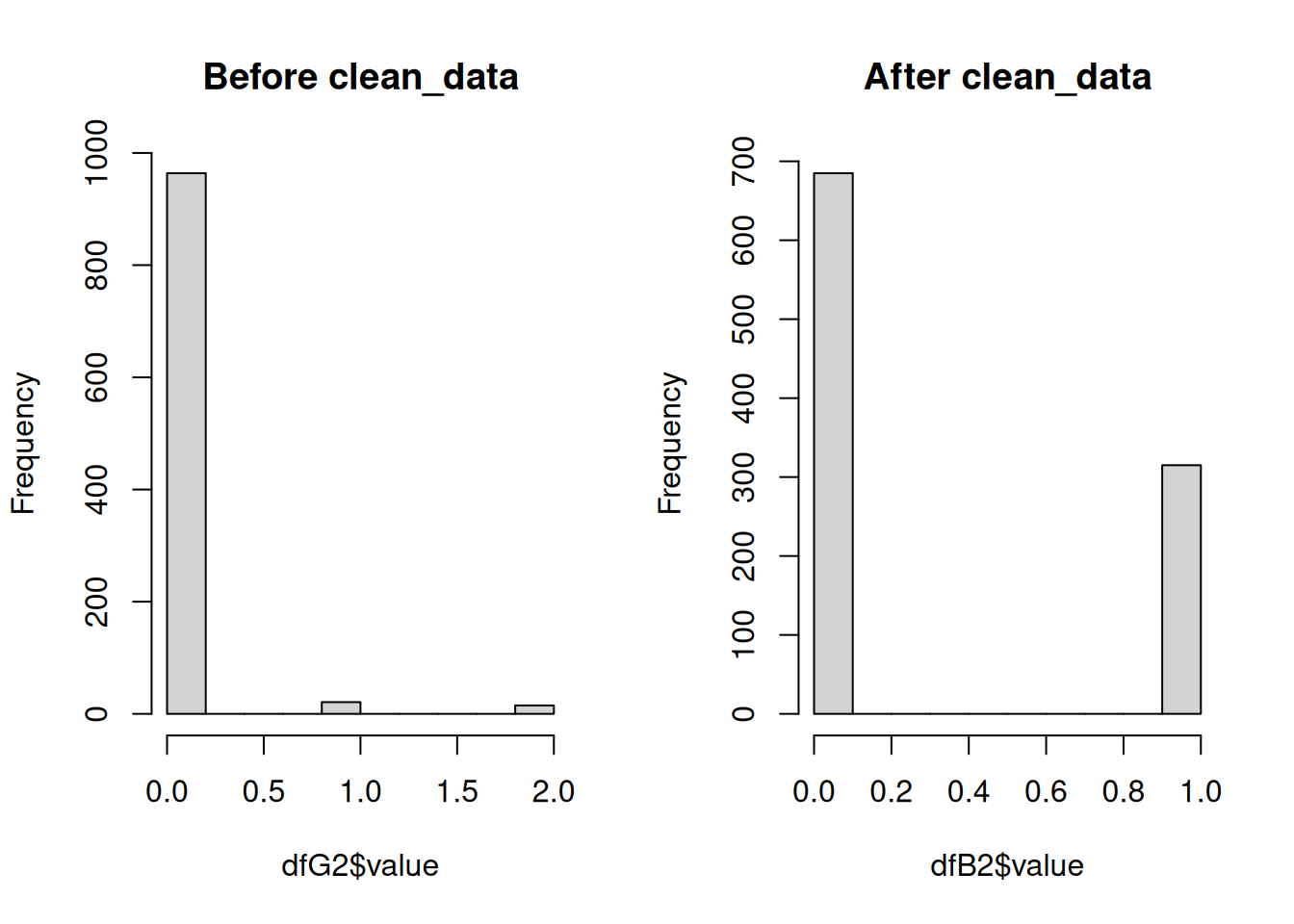
Note that these datasets are random subsets of the complete dataset so the number of presences/absences is not equal in each. These histograms are only to illustrate the shift in range from 0-2 to 0-1.
Finally, we will run remove_corr to remove any correlated environmental covariates before building the model. Position and time (month & year) are retained.
dfC <- remove_corr(dfB, pa_col = 'value', xy_col = c('x', 'y'), month_col = 'month', year_col = 'year')If covariates are removed due to correlation with other covariates, the corresponding column names will be printed in the console or the log file.
The wrapper function makeDF includes all of the functions related to making and cleaning the data frame and provides skip and log file functionalities. This function also makes sure that the combined fisheries raster is loaded and the layers have the appropriate names. Like other wrapper functions, this function also saves the results from each call in the appropriate species-specific folder.
This function is generally not very computationally expensive (takes <10 minutes), unless you are matching a lot of environmental covariates. If you need to perform this operation for a long list of species, the wrapper function is designed to be run in parallel.
load('./Data/MOM6/norm_MOM6_092025.RData') #normalized environmental data needs to be loaded prior to launching the code in parallel
options(future.globals.maxSize = Inf) #remove check for sharing large files so that norm is shared across workers since this is a relatively low memory intensive job otherwise
plan(multisession, workers = 5)
dfs <- future_pmap(list(..1 = args$name, ..2 = args$skip, ..3 = args$mMin, ..4 = args$mMax, ..5 = args$yMin, ..6 = args$yMax), ~ makeDF(name = ..1, skip = ..2, mMin = ..3, mMax = ..4, yMin = ..5, yMax = ..6), .progress = T,  .options = furrr_options(seed = 2025))
plan(sequential)
Building & Predicting Species Distribution Models
Now that the data frames have been constructed and cleaned, you can build the species distribution models. A series of functions are provided to build, perform cross-validation on, evaluate, and extract variable importance from the models for each of the component models for the ensemble: Generalized Additive Model (GAM), MAXENT, Random Forest (RF), Boosted Regression Trees (BRT), sdmTMB.
The first step is building the base model:
mod <- make_sdm(se = dfC, pa_col = 'value', xy_col = c('x', 'y'), month_col = 'month', year_col = 'year', model = model)model is one of the five component models: gam, maxent, rf, brt, sdmtmb or the ensemble (ens). This function first creates the base model and simplifies it as necessary.
The sdm_cv function performs a cross-validation of the model with k = 5.
cv <- sdm_cv(mod = mod, se = dfC, pa_col = 'value', xy_col = c('x', 'y'), month_col = 'month', year_col = 'year', model = model)The predicted values are extracted from the cross-validation output to help build the ensemble and calculate the evaluation metric using the sdm_preds function.
preds <- sdm_preds(cv = cv, model = model)The model is then evaluated using the predicted values. This function can calculate a Root Mean Squared Error (RMSE) or Area under the Curve (AUC).
ev <- sdm_eval(preds = preds, metric = 'auc', model = model)Variable importance for each of the ensemble model components can be extracted from the models:
imp <- sdm_importance(mod = mod, se = dfC, pa_col = 'value', xy_col = c('x', 'y'), month_col = 'month', year_col = 'year', model = model)It is important to note that variable importance from the different models should not be compared without normalizing the values between 0 and 1 as they are all generated using different methods.
The wrapper function makeMods combines the above 5 functions, and includes skip and logging functionality. Like previous wrapper functions, it is easy to launch this in parallel with the furrr functionality.
plan(multisession, workers = 5)
checks <- future_pmap(list(..1 = args$spp, ..2 = args$model, ..3 = args$skip), ~ makeMods(spp = ..1, model = ..2, skip = ..3), .progress = T,  .options = furrr_options(seed = 2025))
plan(sequential)
Where args is the combination of target species and models to be run, along with the flag to enable the skip functionality.
Here, it is important to note that the different models have different memory demands. The GAM, RF, and MAXENT models are the least computationally expensive, followed by BRT. The sdmTMB is the most expensive. Run times will depend on the dataset size, computational resources, and your R environment. Therefore, it is recommended that you generate sdmTMB models in sequence, but all other models can be generated in parallel.
Below are example run times and run conditions for the final model runs for the Northeast CVA2.0 with 36 target species. This includes all of the steps outlined above: 1) building & simplying the model, 2) performing cross validations, and extracting 3) predictions, 4) AUC, and 5) variable importance. All models were run in a remote R terminal, in an environment linked to Intel’s oneAPI, which includes a BLAS library (sdmTMB recommends linking R to an optimized BLAS library to improve runtimes; see the sdmTMB installation guide), with 96 GB of available memory. Final datasets for each species had 100,000+ observations and were not downsampled. The exception to this was the random forest models which perform better with even distributions of presences and absences. All presences were retained and absences were randomly selected across regions in time and space to ensure an even distribution of absences.
| GAM | MAXENT | RF | BRT | sdmTMB | |
|---|---|---|---|---|---|
| Number of Cores | 10 | 12 | 6 | 10 | 1 |
| Total Run Time (hrs) | 15 | 60 | 2 | 26 | 82 |
| Average Model Run Time (hrs)* | 4.2 | 20* | 0.3 | 7.2 | 2.5 |
- Note 1: These are average run times calculated by dividing the total run time by the number of models run per core (36/number of cores). Some individual models were built faster or slower than the times listed due to the number of presences and the complexity of the environmental relationships
- Note 2: The addition of the oneAPI BLAS library increased MAXENT model run times in comparison to previous runs in environments not linked to oneAPI. These previous MAXENT run times in a standard R environment were more similar to GAM run times. However, sdmTMB run times decreased by ~2x (based on small scale tests), but needed to be run in sequence due to memory constraints (yes, even with 96GB of memory, there were memory contrains due to the size of the data set and memory needs of the model), whereas MAXENT models were memory-light enough to be run in parallel.
The function make_predictions will predict the model to a provided timeseries. It has the option to mask off the predictions based on a provided bathymetry raster (bathyR).
load('./Data/MOM6/norm_MOM6_082025.RData') #list of normalized environmental rasterStacks to predict to; number of layers will dictate the time series predicted to
abund <- make_predictions(mod = mod, model = model, rasts = norm, mask = T, bathyR = bathyR, bathy_max = 1000, se = dfC, staticData = './Data/staticVariables_cropped_normZ.RData', xy_col = c('x', 'y'), month_col = 'month', year_col = 'year')
The output will be a rasterStack with the same resolution and number of layers as the time series of environmental data provided.
The wrapper function predictMods loads the necessary data frames and models, and saves the output to the output_rasters directory within the working directory. Similar to other wrapper functions, it also includes skip and logging functionality, and it is written to be easily run in parallel.
plan(multisession, workers = 5)
checks <- future_pmap(list(..1 = args$spp, ..2 = args$model, ..3 = args$skip), ~ predictMods(spp = ..1, model = ..2, skip = ..3), .progress = T,  .options = furrr_options(seed = 2025))
plan(sequential)
It is important to note that for whatever reason, the MAXENT model cannot be predicted in parallel, so it must be run in sequence. However, predicting the models is much quicker and less memory-intensive than making the models themselves.
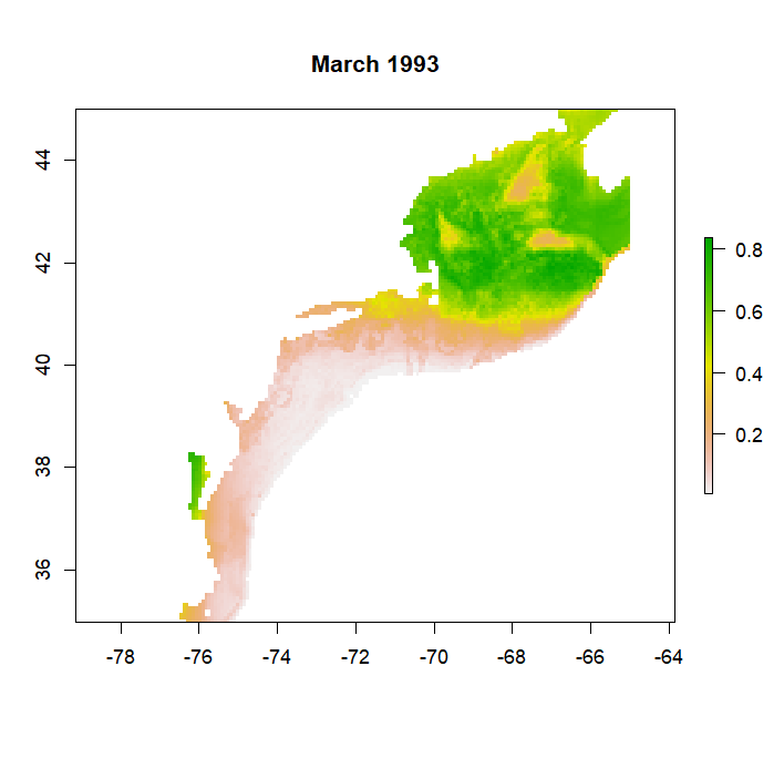
make_predictions will produce a list of rasters, one raster for each time in the time series, that can be converted to a rasterStack with the stack function. Predictions will range between 0 and 1, representing the probability of a species occuring in that grid cell at that time. If mask = T, predictions will be limited to a certain depth range. For example if bathy_max = 1000 then predictions will not be made for areas where the bathymetry is greater than 1000 m as in the example from a GAM model for Atlantic cod below: 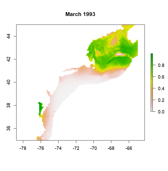
Alternative for sdmTMB Predictions
Regardless of working environment, predictions of sdmTMB models with predictMods can take significant amounts of time. The functions makePredDF and predictSDM offer an alternative workflow similar to predictMods. While predictMods performs the predictions for each timestep, this workflow generates a large dataframe of all environmental raster data across all timesteps, performs the prediction once for all timesteps, then creates the individual rasters for each timestep.
#all arguments are the same as `make_predictions`
allData <- makePredDF(norm, bathyR = bathyR, bathy_max = 1000, staticData = './Data/staticVariables_cropped_normZ.RData', mask = T)
pred <- predict(mod, newdata = allData, type = 'response') #predict everything all at once in a single call
pred$my <- paste(pred$month, pred$year, sep = '.')
abund <- predictSDM(mod = mod, df = pred, staticData = './Data/staticVariables_cropped_normZ.RData') #make into rasters
This workflow can be easily modified to run in a loop across multiple species. It still takes significant amounts of memory (~50GB for the NE Shelf CVA2.0) so running in parallel is not recommended. Luckily, this code takes approximately 25 minutes to run for a single species.
Building & Predicting Ensemble
The ensemble is built using the framework from the EFHSDM package. Here it is included in the make_sdm function:
ens <- make_sdm(model = 'ens', ensembleWeights = weights, ensemblePreds = pds)Where the weights is a vector of model weights produced either by the EFHSDM function MakeEnsemble if using RMSE or another method and pds is a list of prediction outputs from the cross-validation of the models. The weights vector and predictions list must be in the same order to correctly assign weights to predictions.
To predict the ensemble model, the make_predictions function is used:
abund <- make_predictions(model = 'ens', rasts = abds, weights = weights, staticData = NULL, mask = F, bathy_nm = NULL, bathy_max = NULL, se = NULL, month_col = NULL, year_col = NULL, xy_col = NULL)Where abds is a list of predicted rasters from each of the component models. Similar to building the model, the order of the rasters must match the order of the models in the weights vector so that the weights can be assigned appropriately. To predict the ensemble, which is just a weighted average of the component model predictions, only a list of predictor rasters and the model weights are required, so many of the other arguments are set to NULL.
The wrapper function makeEns is provided to combine both the creation and prediction of the ensemble. Creating and predicting the ensemble is fast and quick since it is just performing a weighted average of the existing data, so no skip functionality is provided, but logging functionality remains. This can be run in parallel if desired.
plan(multisession, workers = 5)
checks <- future_pmap(list(..1 = spp.list$Name), ~ makeEns(spp = ..1), .progress = T,  .options = furrr_options(seed = 2025))
plan(sequential)
The resulting list of rasters, which is again a list of raster layers, will be a weighted average of all provided model predictions. So, like the original predictions the values will range between 0 and 1.