This vignette compares fish condition data produced with the
NEesp2::species_condition function to the condition data in
the ecodata package. The
NEesp2::species_condition function was built based on Laurel’s
condition code. This analysis validates whether the function can be
used to automate the workflow for the 2026 SOE.
Create data with NEesp2::species_condition
I’m creating condition data with two different survdat pulls, one from 2024 and one from mid-2025. I think the 2024 pull is the same one used to create the current ecodata condition data; it is on github here. The 2025 pull is a more recent pull that includes data through 2024.
# using a recent survdat pull:
all_condition <- readRDS(here::here("data-raw/condition.rds"))$survdat |>
  NEesp2::species_condition(
    LWparams = NEesp2::LWparams,
    species.codes = NEesp2::species.codes,
    output = "soe"
  )
## Joining with `by = join_by(STRATUM)`
## Joining with `by = join_by(count)`
## Removing 16811 outliers from the data set.
# using an older survdat pull:
load(here::here("data-raw/Survdat_2024.Rdata"))
all_condition_2024 <- survdat |>
  NEesp2::species_condition(
    LWparams = NEesp2::LWparams,
    species.codes = NEesp2::species.codes,
    output = "soe"
  )
## Joining with `by = join_by(STRATUM)`
## Joining with `by = join_by(count)`
## Removing 16239 outliers from the data set.Different numbers of outliers were removed from each dataset. That could be because the more recent survdat pull has some additional data points that are being treated as outliers, or something else is going on.
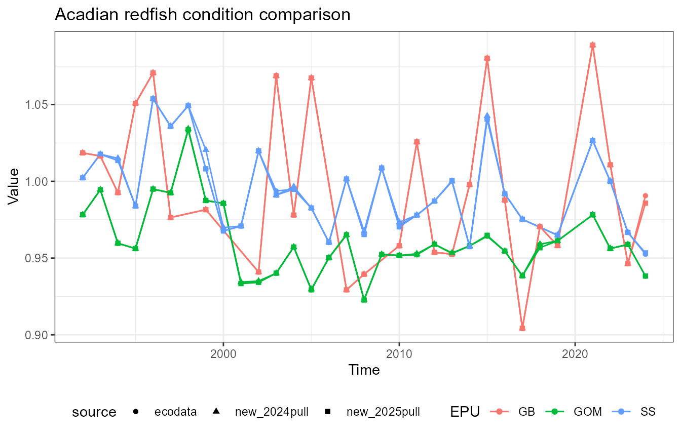
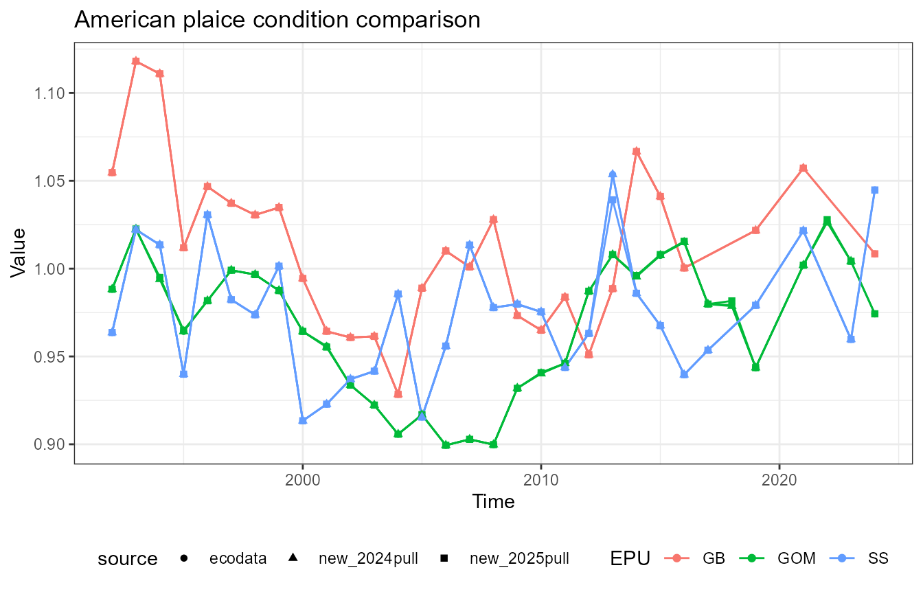
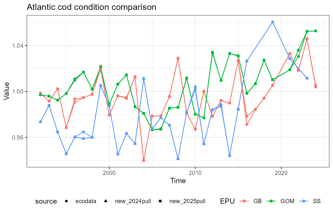
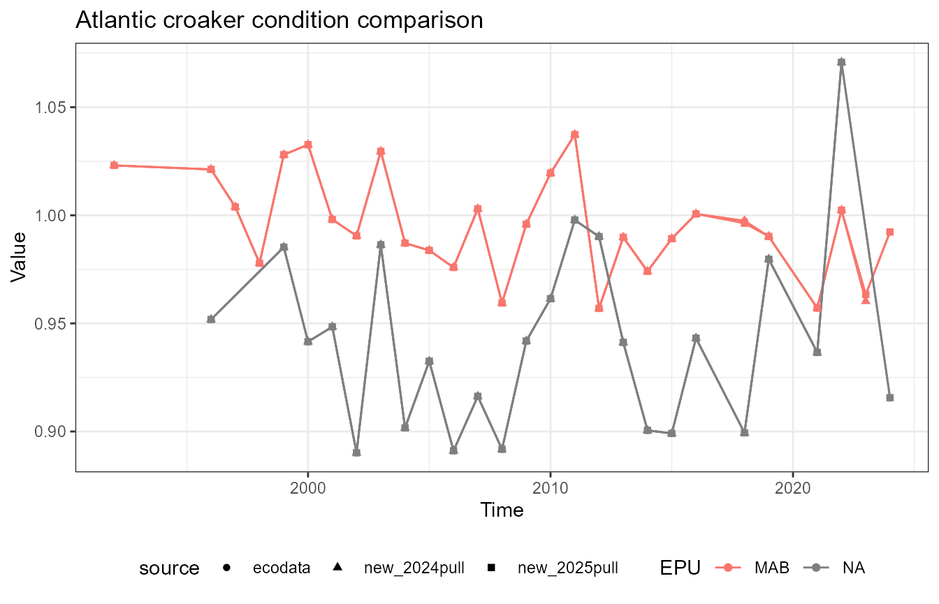
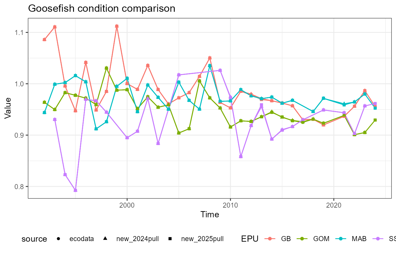
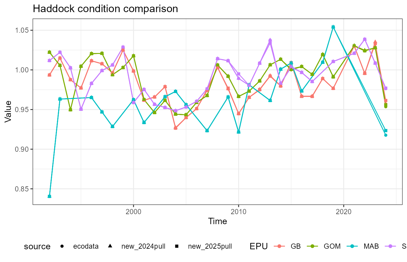
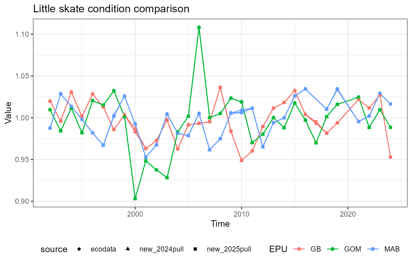
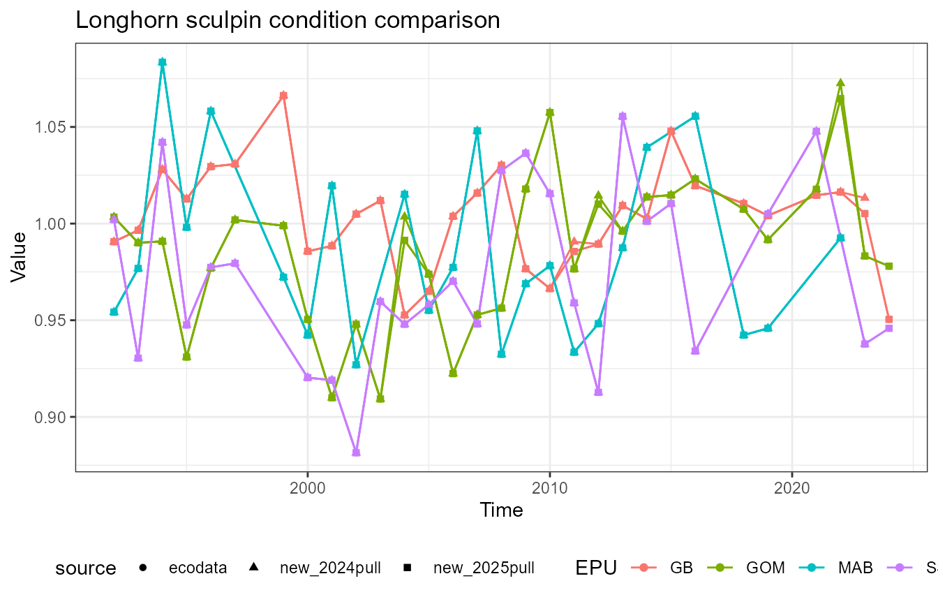
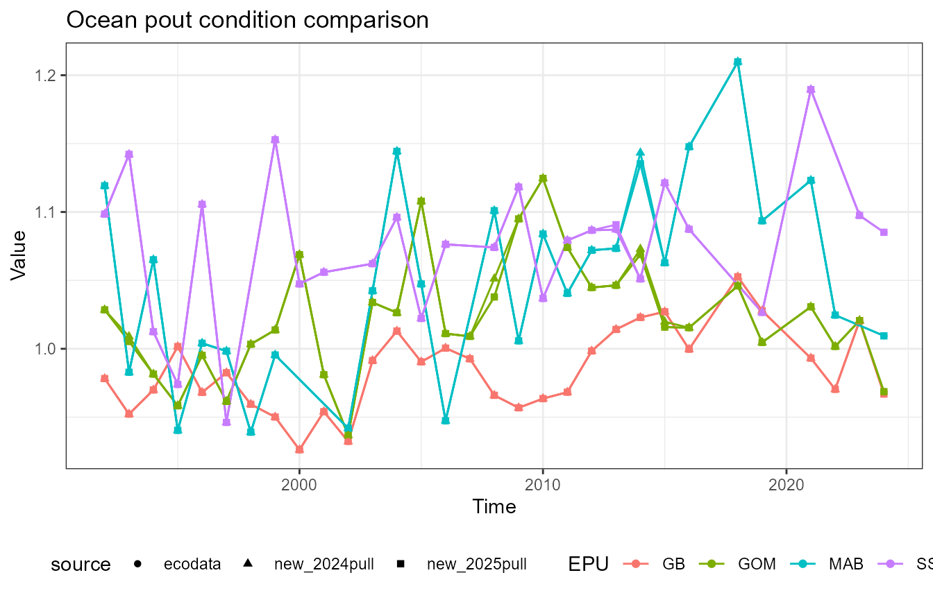
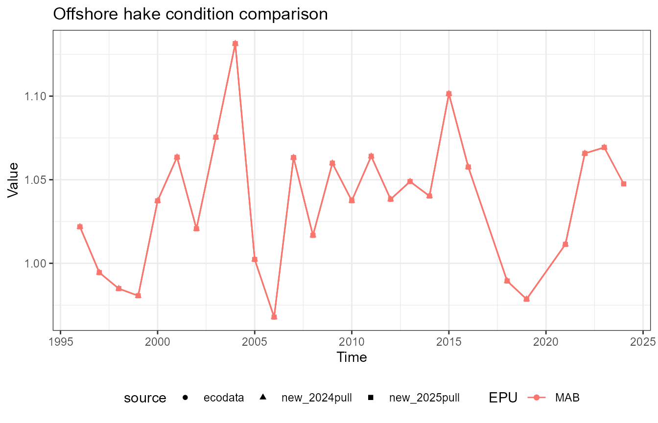
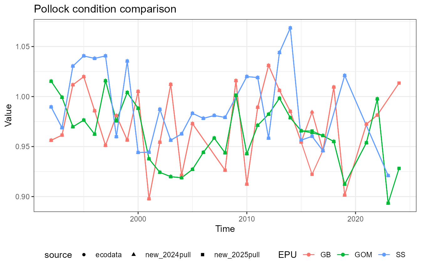
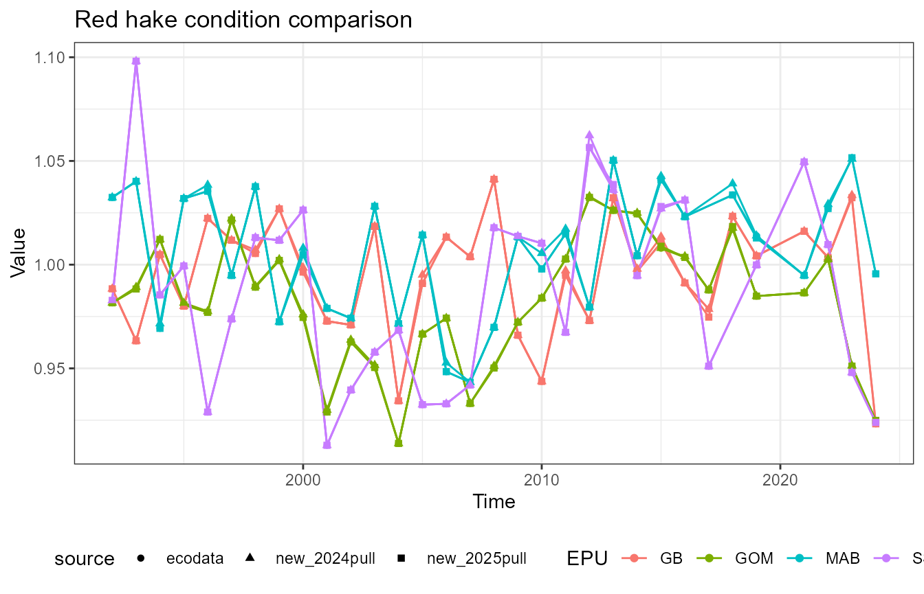
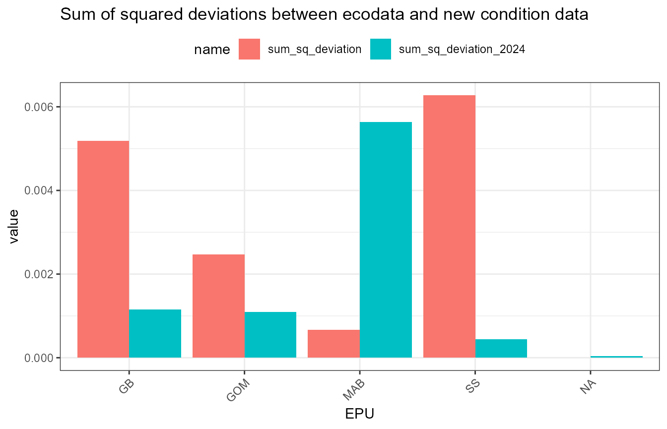
Assess deviations
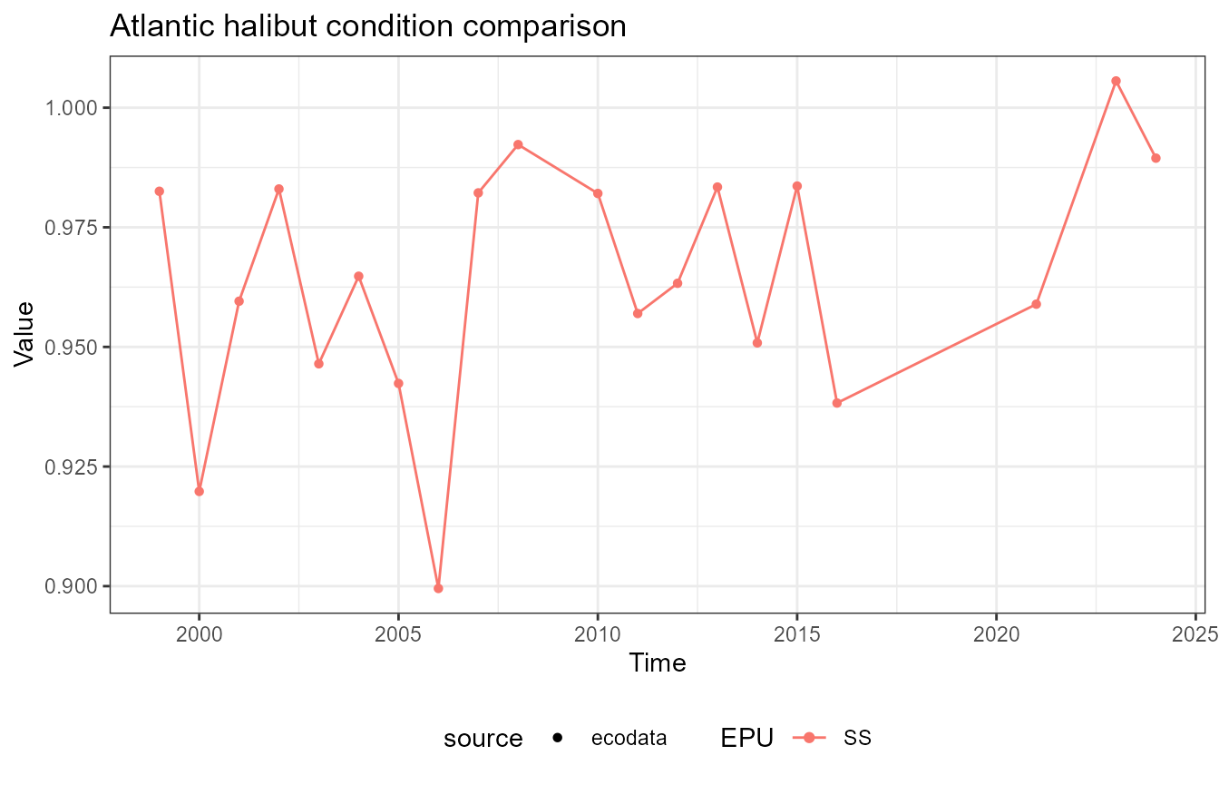
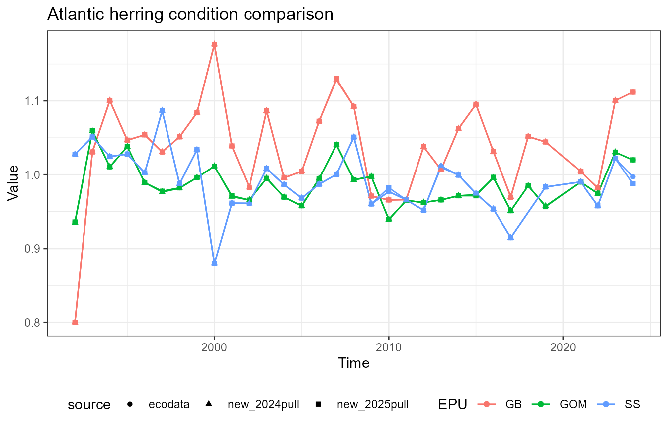
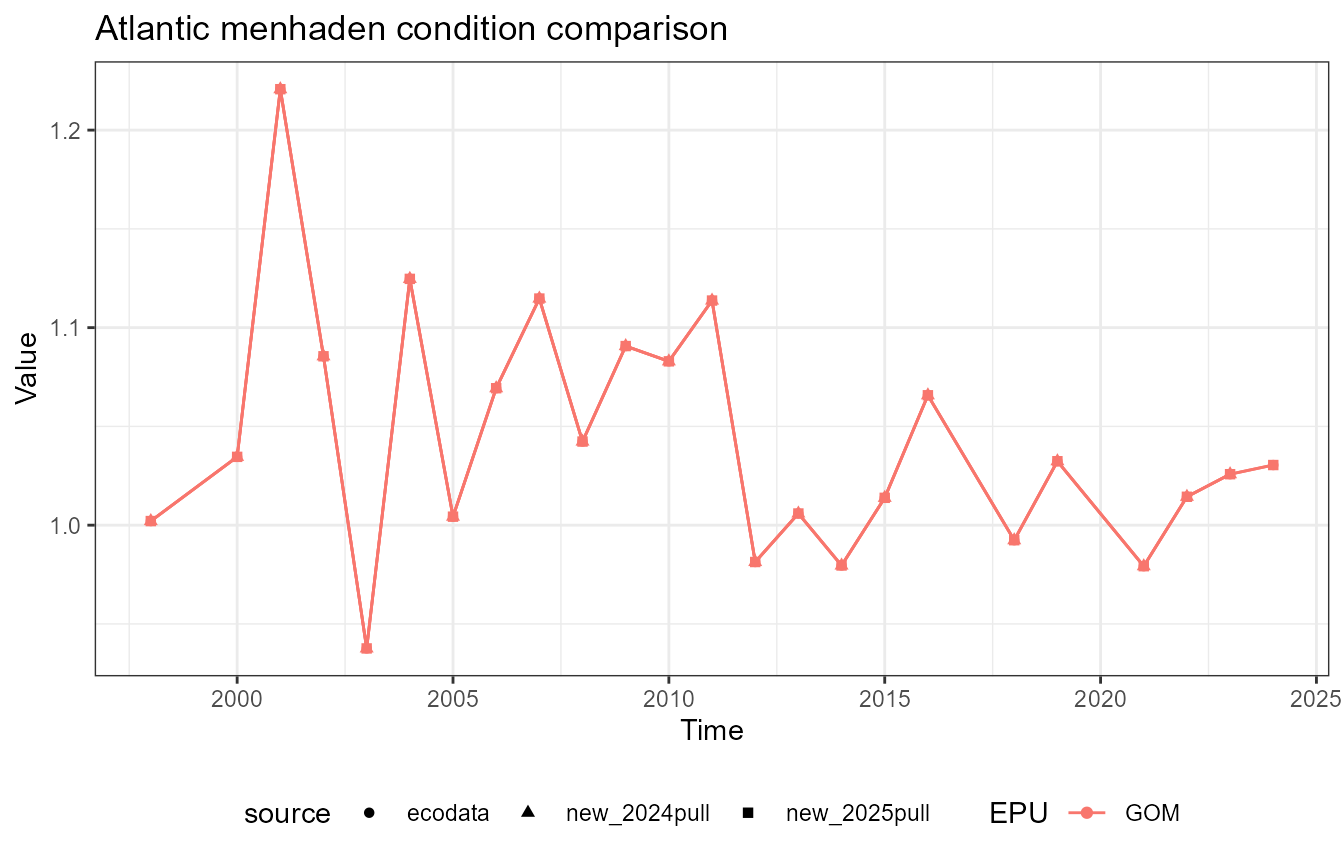
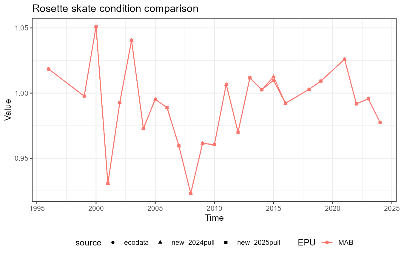
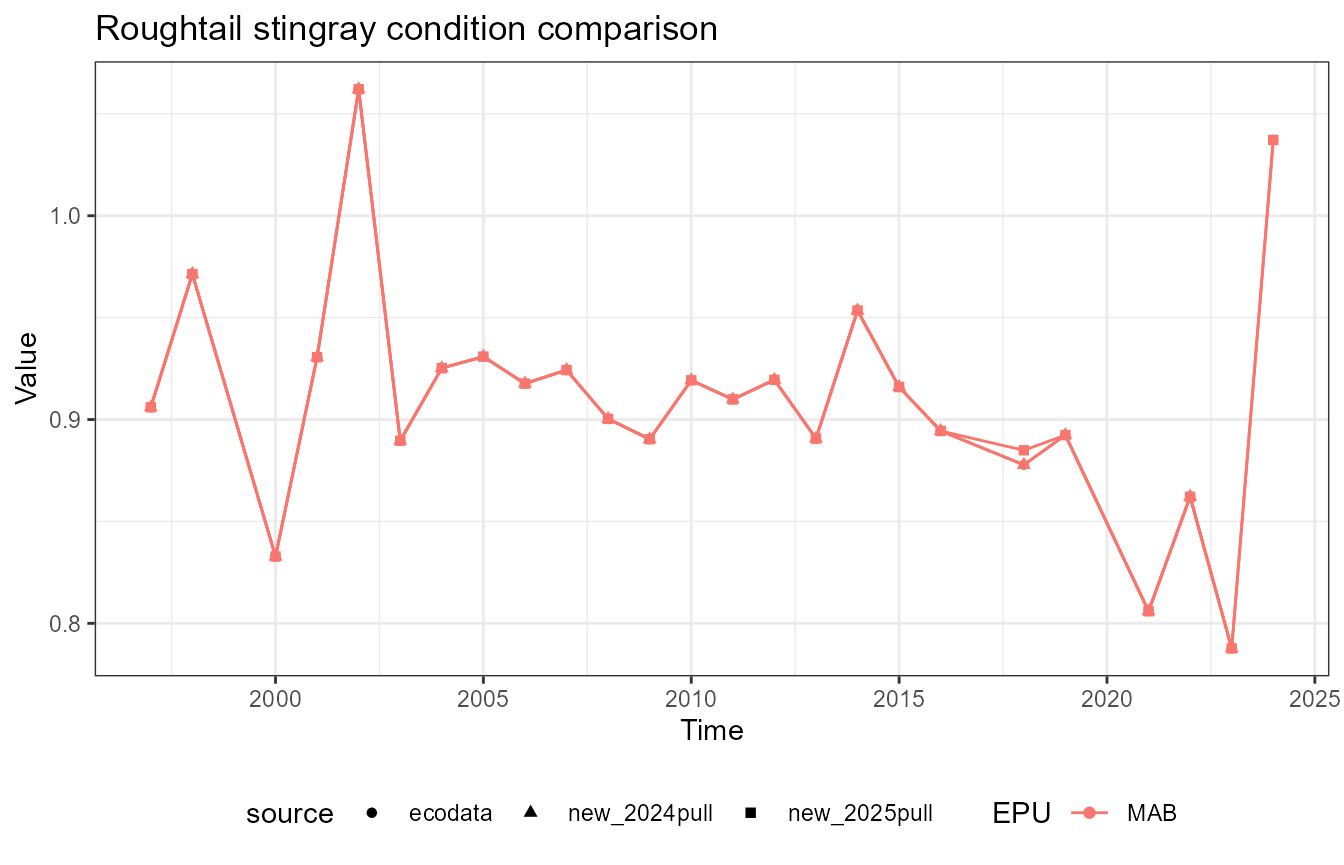
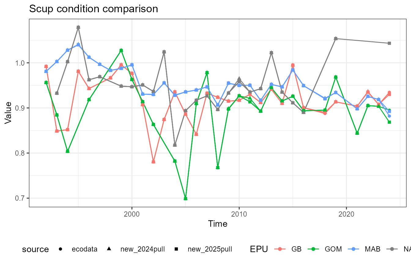
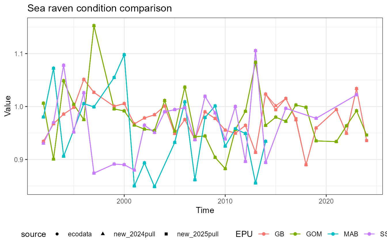
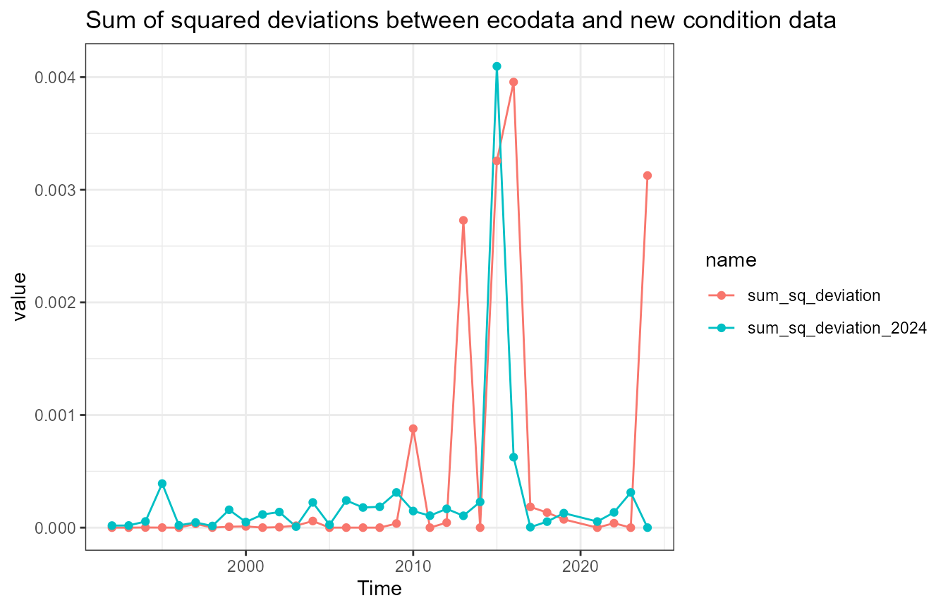
There are some small differences between the newly-calculated data and ecodata. These next analyses look at squared deviations from the ecodata values, to see if there is a systematic bias in any of the data.
full_data <- ecodata::condition |>
  dplyr::rename(ecodata_value = Value) |>
  dplyr::full_join(
    all_condition |>
      dplyr::rename(new_value = Value)
  ) |>
  dplyr::full_join(
    all_condition_2024 |>
      dplyr::rename(new_value_2024 = Value))
## Joining with `by = join_by(Time, Var, EPU, Units)`
## Joining with `by = join_by(Time, Var, EPU, Units)`
dev_data <- full_data |>
  dplyr::mutate(dev_squared = (ecodata_value - new_value)^2,
                dev_squared_2024 = (ecodata_value - new_value_2024)^2)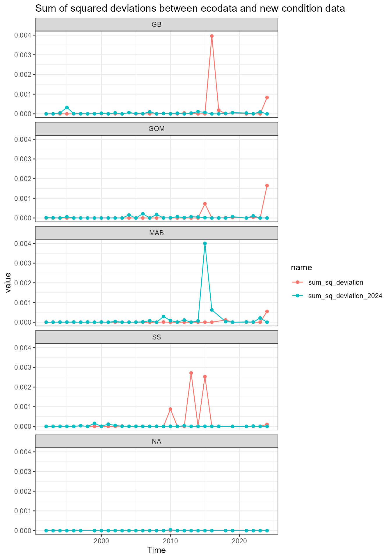
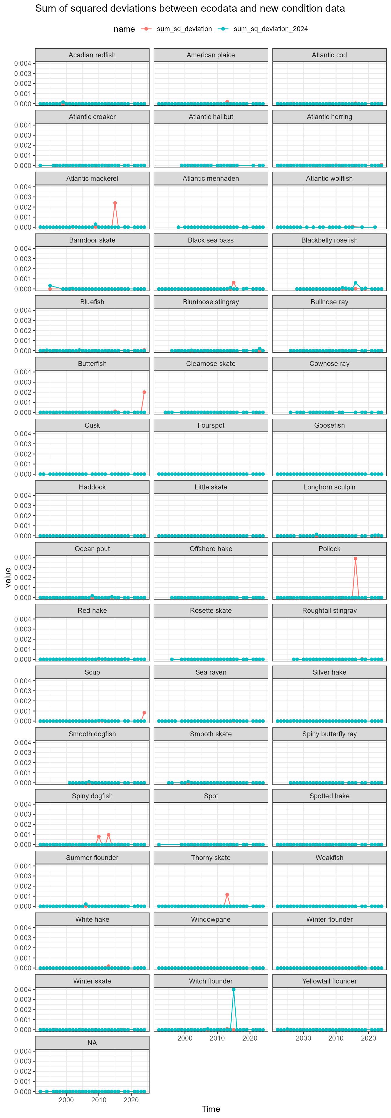
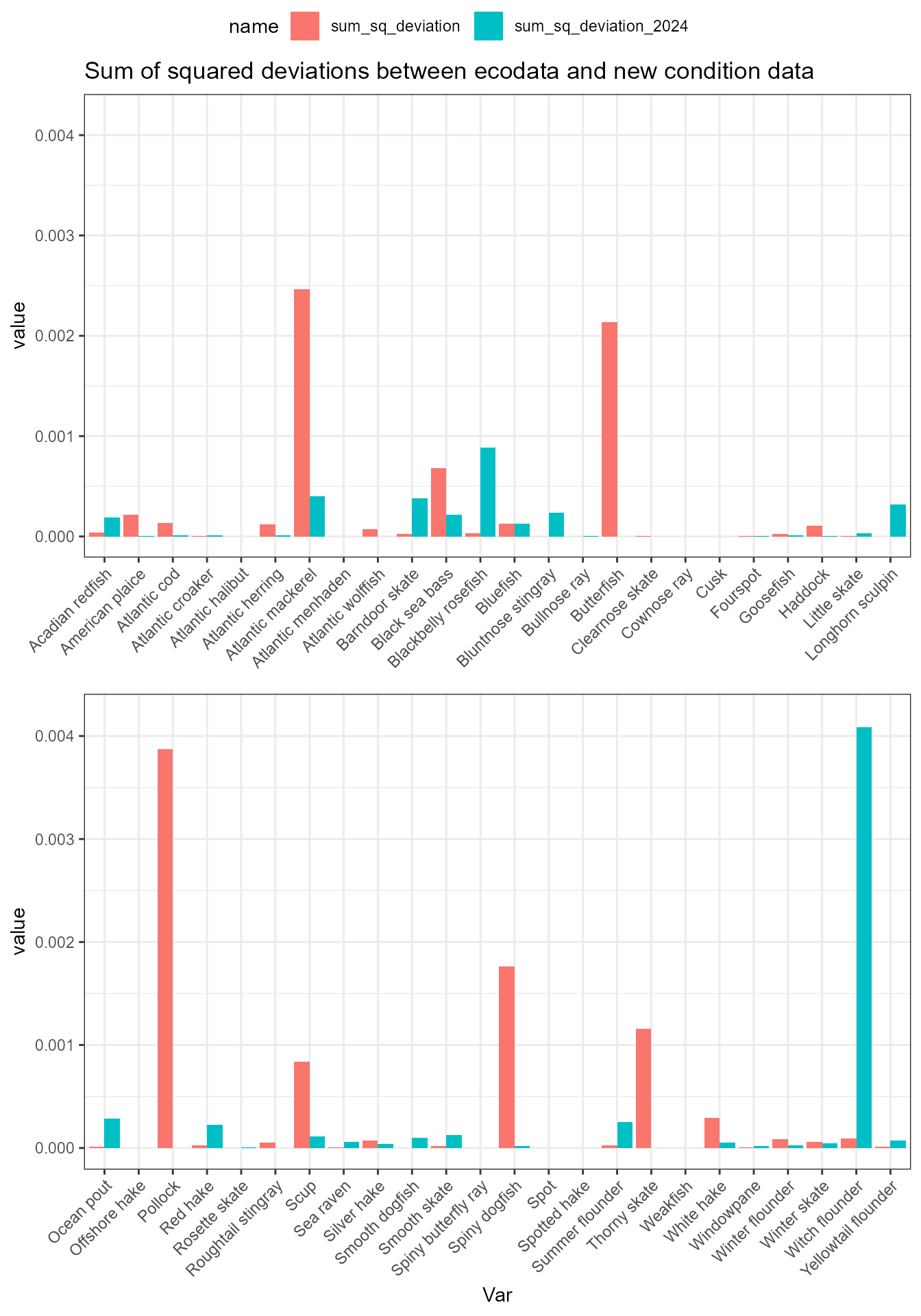
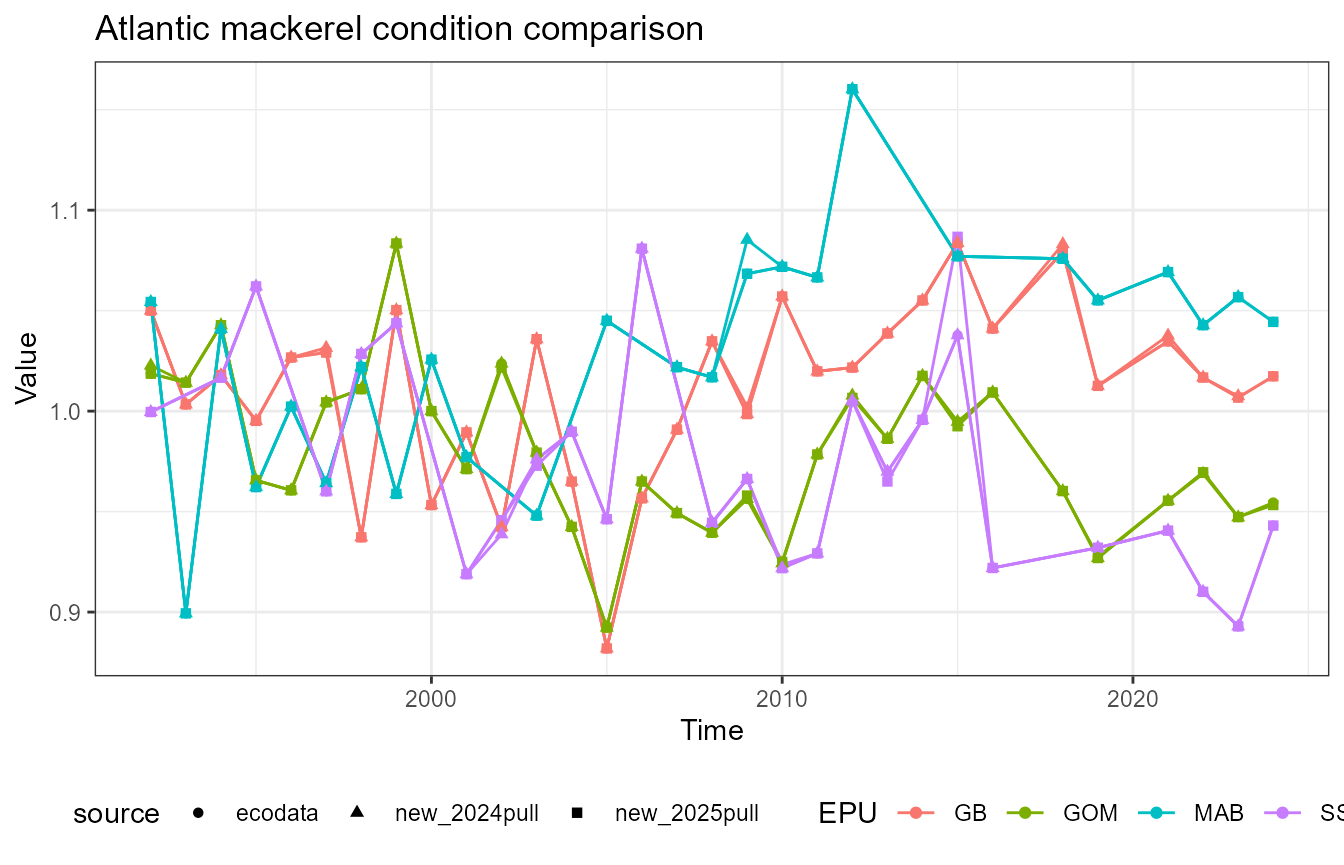
What’s going on with mackerel?
Mackerel has a notable difference in the Scotian Shelf value in 2015. First, recalculate the data:
survdat_2024 <- survdat |>
  dplyr::filter(SVSPP == 121)

survdat_2025 <- readRDS(here::here("data-raw/condition.rds"))$survdat  |>
  dplyr::filter(SVSPP == 121)

cond_comparison <- survdat_2024 |>
  NEesp2::species_condition(
    LWparams = NEesp2::LWparams,
    species.codes = NEesp2::species.codes,
    output = "soe"
  ) |>
  dplyr::mutate(source = "survdat_2024") |>
  dplyr::bind_rows(
    survdat_2025 |>
      NEesp2::species_condition(
        LWparams = NEesp2::LWparams,
        species.codes = NEesp2::species.codes,
        output = "soe"
      ) |>
      dplyr::mutate(source = "survdat_2025")
  ) |>
  dplyr::bind_rows(ecodata::condition |>
                     dplyr::filter(Var == "Atlantic mackerel") |>
                     dplyr::mutate(source = "ecodata"))
## Joining with `by = join_by(STRATUM)`
## Joining with `by = join_by(count)`
## Removing 359 outliers from the data set.
## Joining with `by = join_by(STRATUM)`
## Joining with `by = join_by(count)`
## Removing 400 outliers from the data set.Then plot:
cond_comparison |>
  ggplot2::ggplot(ggplot2::aes(x = Time,
                               y = Value,
                               color = source)) +
  ggplot2::geom_line()+
  ggplot2::geom_point() +
  ggplot2::theme_bw() +
  ggplot2::facet_wrap(~EPU)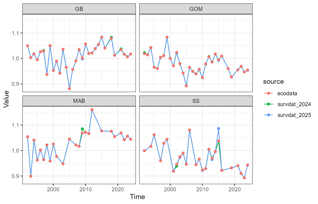
Scotian Shelf in 2015
2024 survdat pull
Take a look at what’s in the 2024 dataset.
mackerel_2024 <- survdat_2024 |>
      dplyr::left_join(NEesp2::strata_epu_key) |>
  dplyr::filter(EPU == "SS",
                YEAR == 2015,
                SEASON == "FALL") |>
  dplyr::select(CRUISE6, STRATUM, LENGTH, LAT, LON, EST_TOWDATE, INDID, INDWT, SEX)

knitr::kable(mackerel_2024)| CRUISE6 | STRATUM | LENGTH | LAT | LON | EST_TOWDATE | INDID | INDWT | SEX |
|---|---|---|---|---|---|---|---|---|
| 201504 | 1340 | 28 | 43.33608 | -66.67322 | 2015-10-17 15:35:26 | 152374 | 0.195 | 2 |
| 201504 | 1340 | 30 | 43.33608 | -66.67322 | 2015-10-17 15:35:26 | 152338 | 0.270 | 1 |
| 201504 | 1340 | 31 | 43.33608 | -66.67322 | 2015-10-17 15:35:26 | 152357 | 0.315 | 2 |
| 201504 | 1340 | 32 | 43.33608 | -66.67322 | 2015-10-17 15:35:26 | 152247 | 0.293 | 1 |
| 201504 | 1340 | 32 | 43.33608 | -66.67322 | 2015-10-17 15:35:26 | 152344 | 0.320 | 1 |
| 201504 | 1340 | 33 | 43.83454 | -66.73564 | 2015-10-18 01:38:50 | 153828 | 0.336 | 2 |
| 201504 | 1351 | 17 | 44.27302 | -66.70087 | 2015-10-18 08:31:51 | 154973 | 0.051 | 2 |
| 201504 | 1351 | 18 | 44.27302 | -66.70087 | 2015-10-18 08:31:51 | 154967 | 0.060 | 2 |
| 201504 | 1340 | 34 | 44.03344 | -66.94544 | 2015-10-18 14:47:12 | 156565 | 0.455 | 2 |
| 201504 | 1340 | 31 | 43.88735 | -67.20750 | 2015-10-18 17:30:51 | 157004 | 0.335 | 2 |
| 201504 | 1340 | 33 | 43.88735 | -67.20750 | 2015-10-18 17:30:51 | 157001 | 0.410 | 1 |
| 201504 | 1340 | 33 | 43.88735 | -67.20750 | 2015-10-18 17:30:51 | 156998 | 0.365 | 1 |
2025 survdat pull
Take a look at what’s in the 2025 dataset.
mackerel_2025 <- survdat_2025 |>
      dplyr::left_join(NEesp2::strata_epu_key) |>
  dplyr::filter(EPU == "SS",
                YEAR == 2015,
                SEASON == "FALL") |>
  dplyr::select(CRUISE6, STRATUM, LENGTH, LAT, LON, EST_TOWDATE, INDID, INDWT, SEX)

knitr::kable(mackerel_2025)| CRUISE6 | STRATUM | LENGTH | LAT | LON | EST_TOWDATE | INDID | INDWT | SEX |
|---|---|---|---|---|---|---|---|---|
| 201504 | 1340 | 33 | 43.83454 | -66.73564 | 2015-10-18 02:38:50 | 153828 | 0.336 | 2 |
| 201504 | 1351 | 17 | 44.27302 | -66.70087 | 2015-10-18 09:31:51 | 154973 | 0.051 | 2 |
| 201504 | 1351 | 18 | 44.27302 | -66.70087 | 2015-10-18 09:31:51 | 154967 | 0.060 | 2 |
| 201504 | 1340 | 34 | 44.03344 | -66.94544 | 2015-10-18 15:47:12 | 156565 | 0.455 | 2 |
| 201504 | 1340 | 31 | 43.88735 | -67.20750 | 2015-10-18 18:30:51 | 157004 | 0.335 | 2 |
| 201504 | 1340 | 33 | 43.88735 | -67.20750 | 2015-10-18 18:30:51 | 157001 | 0.410 | 1 |
| 201504 | 1340 | 33 | 43.88735 | -67.20750 | 2015-10-18 18:30:51 | 156998 | 0.365 | 1 |
Looks like the October 17, 2015 tow is missing from the 2025 pull.
Double check the input data:
test_survdat <- readRDS(here::here("data-raw/condition.rds"))$survdat  |>
  dplyr::filter(stringr::str_detect(EST_TOWDATE, "2015-10-17"))

test_survdat$SVSPP |> unique() |> sort()
## [1] 15 22 27 28 32 35 72 73 74 75 76 77 84 101 102 106 107 131 155
## [20] 156 163 193 197 301 312 502Mackerel isn’t in there (SVSPP 121).
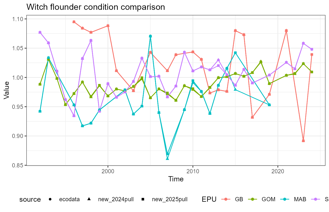
What’s going on with witch flounder?
Witch flounder has a notable difference in the Mid-Atlantic Bight value in 2015. First, recalculate the data:
survdat_2024 <- survdat |>
  dplyr::filter(SVSPP == 107)

survdat_2025 <- readRDS(here::here("data-raw/condition.rds"))$survdat  |>
  dplyr::filter(SVSPP == 107)

cond_2024 <- survdat_2024 |>
  NEesp2::species_condition(
    LWparams = NEesp2::LWparams,
    species.codes = NEesp2::species.codes,
    record_outliers = TRUE,
    output = "soe"
  )
## Joining with `by = join_by(STRATUM)`
## Joining with `by = join_by(count)`
## Removing 390 outliers from the data set.
cond_2025 <- survdat_2025 |>
      NEesp2::species_condition(
        LWparams = NEesp2::LWparams,
        species.codes = NEesp2::species.codes,
    record_outliers = TRUE,
        output = "soe"
      )
## Joining with `by = join_by(STRATUM)`
## Joining with `by = join_by(count)`
## Removing 424 outliers from the data set.
cond_comparison <- cond_2024$condition |>
  dplyr::mutate(source = "survdat_2024") |>
  dplyr::bind_rows(cond_2025$condition|>
      dplyr::mutate(source = "survdat_2025")) |>
  dplyr::bind_rows(ecodata::condition |>
                     dplyr::filter(Var == "Witch flounder") |>
                     dplyr::mutate(source = "ecodata"))
Plot the data:
cond_comparison |>
  ggplot2::ggplot(ggplot2::aes(x = Time,
                               y = Value,
                               color = source)) +
  ggplot2::geom_line()+
  ggplot2::geom_point() +
  ggplot2::theme_bw() +
  ggplot2::facet_wrap(~EPU)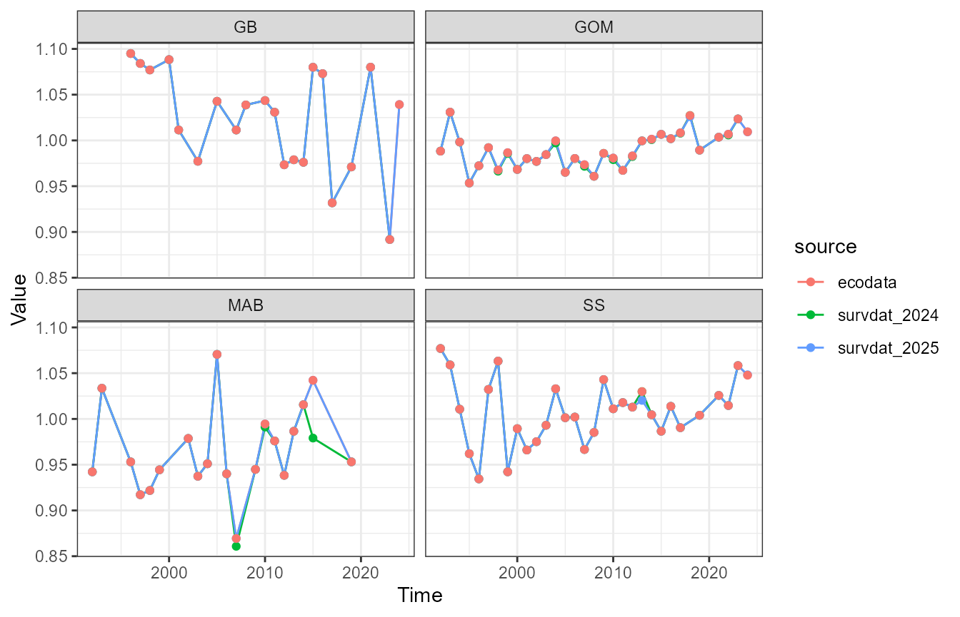
Mid-Atlantic Bight in 2015
2024 survdat pull
witch_2024 <- survdat_2024 |>
      dplyr::left_join(NEesp2::strata_epu_key) |>
  dplyr::filter(EPU == "MAB",
                YEAR == 2015,
                SEASON == "FALL") |>
  dplyr::select(CRUISE6, STRATUM, LENGTH, LAT, LON, EST_TOWDATE, INDID, INDWT, SEX)

knitr::kable(witch_2024)| CRUISE6 | STRATUM | LENGTH | LAT | LON | EST_TOWDATE | INDID | INDWT | SEX |
|---|---|---|---|---|---|---|---|---|
| 201504 | 1720 | 22 | 38.47240 | -73.50522 | 2015-09-02 18:17:17 | 2537 | 0.046 | 1 |
| 201504 | 1020 | 30 | 39.91528 | -73.08380 | 2015-09-13 01:45:02 | 59094 | 0.152 | 1 |
| 201504 | 1070 | 29 | 40.21977 | -71.00322 | 2015-09-16 22:04:58 | 76958 | 0.162 | 1 |
| 201504 | 1060 | 34 | 40.49986 | -70.79864 | 2015-09-17 02:44:47 | 78183 | 0.237 | 1 |
2025 survdat pull
witch_2025 <- survdat_2025 |>
      dplyr::left_join(NEesp2::strata_epu_key) |>
  dplyr::filter(EPU == "MAB",
                YEAR == 2015,
                SEASON == "FALL") |>
  dplyr::select(CRUISE6, STRATUM, LENGTH, LAT, LON, EST_TOWDATE, INDID, INDWT, SEX)

knitr::kable(witch_2025)| CRUISE6 | STRATUM | LENGTH | LAT | LON | EST_TOWDATE | INDID | INDWT | SEX |
|---|---|---|---|---|---|---|---|---|
| 201504 | 1720 | 22 | 38.47240 | -73.50522 | 2015-09-02 19:17:17 | 2537 | 0.046 | 1 |
| 201504 | 1020 | 30 | 39.91528 | -73.08380 | 2015-09-13 02:45:02 | 59094 | 0.152 | 1 |
| 201504 | 1070 | 29 | 40.21977 | -71.00322 | 2015-09-16 23:04:58 | 76958 | 0.162 | 1 |
| 201504 | 1060 | 34 | 40.49986 | -70.79864 | 2015-09-17 03:44:47 | 78183 | 0.237 | 1 |
The two datasets are the same. Is the discrepancy caused by outliers being removed?
Outlier analysis
Outliers in the 2024 data:
# cond_comparison |>
#   dplyr::filter(Time == 2015) |>
#   dplyr::arrange(EPU)

cond_2024$outliers |>
  dplyr::filter(YEAR == 2015)  |>
  dplyr::select(CRUISE6, STRATUM, LENGTH, LAT, LON, EST_TOWDATE, INDID, INDWT, SEX) |>
      dplyr::left_join(NEesp2::strata_epu_key) |>
  dplyr::filter(EPU == "MAB") |>
  dplyr::arrange(INDWT) |>
  nrow()
## [1] 0There are no outliers in the 2024 data set.
Outliers in the 2025 data:
cond_2025$outliers |>
  dplyr::filter(YEAR == 2015)  |>
  dplyr::select(CRUISE6, STRATUM, LENGTH, LAT, LON, EST_TOWDATE, INDID, INDWT, SEX) |>
        dplyr::left_join(NEesp2::strata_epu_key) |>
  dplyr::filter(EPU == "MAB") |>
   dplyr::arrange(INDWT) |>
knitr::kable()| CRUISE6 | STRATUM | LENGTH | LAT | LON | EST_TOWDATE | INDID | INDWT | SEX | EPU |
|---|---|---|---|---|---|---|---|---|---|
| 201504 | 1720 | 22 | 38.4724 | -73.50522 | 2015-09-02 19:17:17 | 2537 | 0.046 | 1 | MAB |
The 2025 data set has one outlier. This data point is considered an outlier in the 2025 data, but not in the 2024 data, which causes the difference in the 2015 condition value in the MAB.
Take a look at the outlier:
plt <- survdat_2024 |>
  dplyr::mutate(source = "2024") |>
  dplyr::bind_rows(
    survdat_2025 |>
      dplyr::mutate(source = "2025")
  ) |>
  dplyr::filter(SEASON == "FALL",
                !is.na(LENGTH),
                !is.na(INDWT)) |>
  ggplot2::ggplot(ggplot2::aes(x = LENGTH,
                               y = INDWT,
                               color = source,
                               shape = source)) +
  ggplot2::geom_point(cex = 2,
                      alpha = 0.5) +
  ggplot2::theme_bw()

plt +
  ggplot2::geom_point(ggplot2::aes(x = LENGTH,
                               y = INDWT),
                      data = witch_2025[1,],
                      inherit.aes = FALSE,
                      color = "black")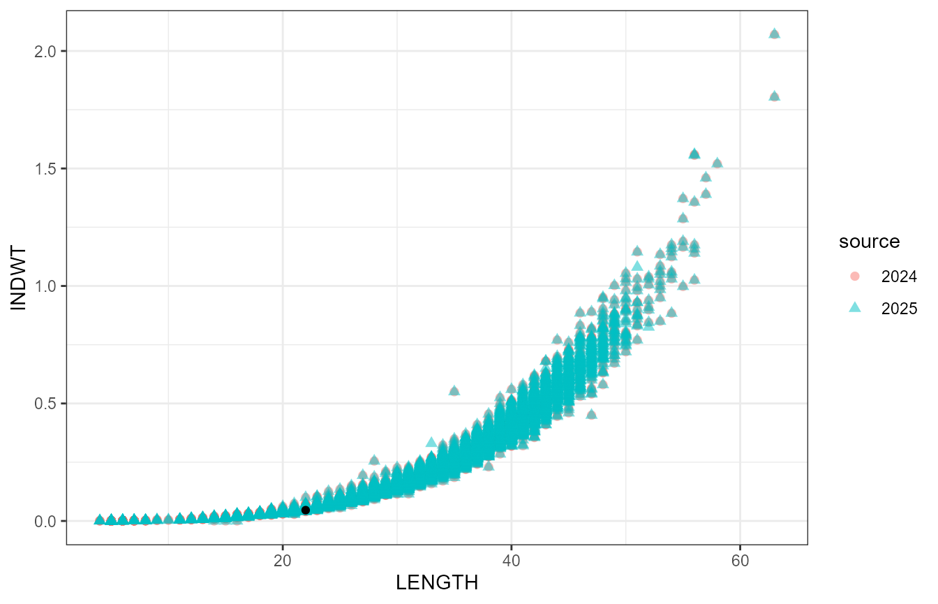
The black point is the outlier, as defined by having a relative condition < 2SD below the species’ mean relative condition over all years. I don’t think it should be treated as an outlier.
Summary
Some discrepancies are caused by differences in the underlying survdat data. These should be validated against the current data in the NEFSC database. Other discrepancies are caused by differences in outlier removal. Since outliers are defined based on standard deviations, the addition of more data changes the outlier cutoff. We would need to update the outlier removal method to be more consistent over time if we want to avoid this issue in the future.